A couple weeks ago, I was introduced to Desmos.

Desmos is an online graphing calculator. It can plot lots of different types of functions in a really intuitive way. But its real hook is that all of its graphs are interactive. You can define a variable and Desmos will automatically make a slider so you can change that variable's value and see the result in real time. You can even click and drag points on the graph itself. It makes math so tangible and I love it.

Within the first day of using Desmos, an idea entered my mind that I couldn't shake: if Desmos can make 2D graphs so interactive, could it do the same for 3D?

It turns out, the answer is yes.

Making this happen pushed the features of Desmos to the absolute limit. In this article I want to give a more detailed breakdown of how it's done.

Before we get into Desmos itself, we need to cover the math of 3D rendering.

How does the math work?

At a high level, 3D rendering is just a long series of transformations. We want to take a set of points in 3D space and move, rotate, stretch, and flatten them until they're all where we want them in a 2D image. Before we can dig into the details of each transformation, though, we need to look at the big picture.

Let's start with what we know:

• We're going to have a model to render, like the cube in my example. For me, the model is just a list of points in 3D space. The model can have its own position and rotation in the scene that we're going to render. (In my renderer, I only have controls for rotation.)
• We're also going to have a camera, which defines the point of view of the image. The camera will have its own position and rotation, plus some camera-specific stuff like a field of view.

So that's the information we start with. We end with 2D points laid out so that they form an image from the camera's point of view. How we get from start to finish goes through four stages. I'll call those stages model space, world space, camera space, and projection space.

Model space is our starting point. The points of our model are centered around the origin (or the center of our world). When we create a model, we define all of its points in model space.

In world space, everything is placed where it belongs in our 3D scene. You can see that the model is rotated to a new orientation, and our camera has been moved and rotated to point at it.

In camera space, we shift everything in the scene so that the camera is at the center, pointing forward. We're effectively moving everything to the camera's point of view. This might seem like a surprising step, but it makes the next stage much easier.

Finally, in projection space, we flatten the world down from three dimensions to two. This is where the camera's field of view comes into play, because we use it to give our final image a sense of perspective.

Once we're in projection space, we are working in two dimensions! All that remains is to plot those 2D points and we have ourselves an image.

Now let's get into the nitty-gritty of how to do this.

Some small prerequisites

Graphics math is all about vectors and matrices. In our case, we use vectors to represent the points of our model and matrices to represent ways of transforming them. If you've never encountered vectors before, the best way to get up to speed is 3blue1brown's excellent Essence of Linear Algebra series on Youtube. For what we're doing, you only need the information from the first four videos, which should take you less than an hour to get through.

You really should watch those videos; they explain the basics far better than I can. But here's my whirlwind summary of the parts we'll be using:

• We'll use vectors to represent the points of our model. Although our points are all three-dimensional, we actually will be using four-dimensional vectors to represent them. The first three components will be the x, y, and z of the point as you would expect. The last component of the vector will just be the number 1. For example, a 3D point with an X position of 1, a Y position of 2, and a Z position of 3 would look like:

  

• We'll use matrices to represent transformations. I'm omitting the details, but for example, a matrix that rotates vectors by 90° around the y axis would look like:

  

• Multiplying a vector by a matrix transforms that vector accordingly. For example, here is what it looks like to rotate our example vector by 90 degrees around the Y axis, color-coded so it's easier to follow:

  

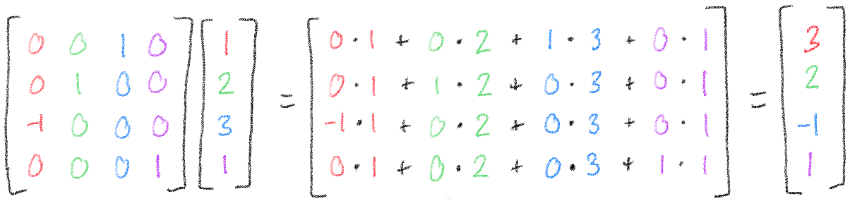
  If you have never seen this kind of multiplication before, I recommend trying to see how this one fits together. I'll be glossing over some details throughout this article, but parts of it will still make more sense if you have an idea of how this works.

Also, it probably seems strange to use four-dimensional vectors to represent three-dimensional data, but the reason we do it is pretty interesting. The short version is that we can do a clever trick with a fourth dimension to do some transformations that wouldn't otherwise be possible with matrices. The long version will have to wait for another blog post, but if you're impatient, just look up "homogeneous coordinates".

Model space to world space

The first major transformation is going from model space to world space, where the model gets placed into our overall scene. For my renderer, I chose to do just two rotations, since it made the controls easy. I first rotate the model about the X axis, then about the Y axis - you could do the rotations in a different order, but I liked the results I got with that.

Order matters when multiplying vectors and matrices - we always have the matrix on the left and the vector on the right. But this means that a series of transformations gets built up from right to left, instead of left to right as you might expect. To rotate first by X, then by Y, our equation will look like:

A more general-purpose renderer could add lots more to this step - for example, moving the model around in space, rotating along the Z axis, or scaling it up and down. But a little rotation is enough for now.

World space to camera space

We now have to go from world space to camera space, where the camera is at the center. This is very similar to our last step - but there's a twist.

In the last step, our model started at the origin and we moved it somewhere else. This time, our camera is somewhere else and we want to move it back to the origin. This means that we need to find the transformations that would move the camera to the right place, but then do those transformations in reverse.

To show you why this works, let's step back to two dimensions for a bit. Say we want to shift everything in this picture so that the blue triangle is at the origin. It's at the coordinates \(\begin{bmatrix}1 \ 2\end{bmatrix}\). What transformation do we have to do to put it back?

Since the triangle is right by 1 and up by 2, we need to shift everything left by 1 and down by 2. If the coordinates are \(\begin{bmatrix}1 \ 2\end{bmatrix}\), the transformation we need to do is \(\begin{bmatrix}-1 \ -2\end{bmatrix}\).

This applies to rotations too. If the triangle were rotated by by 30 degrees, we would need to rotate it by -30 degrees to undo the rotation.

Let's jump back to our scene now. The camera in our scene has been moved and rotated. The sequence of transformations to move it to the right place is: Rotate X, Rotate Y, Move. To undo those transformations, we do: Move, Rotate Y, Rotate X.

Our equation to move a vector \(\vec{v}\) from world space to camera space is therefore:

And our whole equation so far is:

Camera space to projection space

There's just one more transformation to make, and that is the perspective projection. It is finally time to convert our 3D points into 2D points, but we need to make sure that the camera's perspective is taken into account. But what does that perspective actually mean for our image?

Let's look at the camera's field of view. These dashed lines represent the boundaries of what the camera can see, and I've highlighted a certain chunk of the camera's view for us to look at. You can see it sort of looks like a pyramid with the top chopped off - this shape is called a frustum. Also notice in this picture that we have drawn a couple squares on each end of the frustum, both the same size.

Let's think about what those squares would look like in our final image. We know that things closer to the camera appear bigger, and things farther from the camera appear smaller, so whatever transformation we do should have that effect on those squares.

The trick to perspective projection is to imagine stretching and squishing the ends of the frustum so that they’re the same size. When we’re done, we no longer have a frustum - we have a perfectly rectangular box.

You can see that this stretching motion made the blue front square bigger and the red back square smaller! Now we can flatten the points down along the Z axis to be left with a lovely 2D image:

And that's it! Now that we have a set of 2D points, we can simply tell Desmos to plot them and we're done.

Our final equation is therefore:

Doing linear algebra in Desmos

It's all well and good that we know the math - but now we need to implement the math in Desmos!

In order to render an image, we need to figure out how to represent both vectors and matrices in Desmos. More precisely, we need to represent vectors and multiplying those vectors by matrices.

We'll start with vectors, since our model is basically nothing but a list of vectors anyway. Desmos actually doesn't have a lot of features for us to choose from here - the only thing that really works is a list.

A list in Desmos looks like a list of things inside square brackets and separated by commas. For example, we could make a list of numbers like \([1, 2, 3]\), or a list of 2D points like \(\left[(1, 1), (2, -1), (-1, -1)\right]\).

A vector as we use it is basically just a list of numbers, so you'd think Desmos's lists would work well for this. But Desmos has an important limitation that will make life more difficult: it does not allow lists of lists. So while it can do a list of numbers, or a list of points, we couldn't, for example, do the following:

This is a problem for us, because if we represent vectors with lists, but our model is a list of vectors, then we have a list of lists. There aren't any other built-in features of Desmos to use, so let's explore a couple workarounds:

• Workaround 1: separate lists for each component

  Perhaps we could just put all the x's in one list, all the y's in another, and all the z's in another still. Then we would only have three lists, and maybe we could make that work with our matrix math later on.

  

  Unfortunately, this doesn't work because we actually end up with a list of lists again as soon as we try to use these. The reason why is pretty simple - mathematical functions can take many values as input, but produce only one value as output. A matrix-vector multiplication function would need to take separate lists of x, y, and z, but also produce three lists with the x, y, and z results. If Desmos allowed lists of lists, we could return a list containing all three. But it doesn't, so we can't. We'll need to try another approach.

• Workaround 2: pack everything into one big list

  Following from the last workaround, we know that the result of our functions has to be a single value. So it sounds like we need a way of packing all of our x's, y's, and z's into a single list. The simplest way would be to simply go \([x, y, z, x, y, z, \ldots]\). Luckily, it turns out that this will work!

Now we need to figure out what it looks like to do multiplication with a giant, packed list of points. This gets a little strange. We'll stick to two dimensions for the sake of this example, but the technique we're about to explore works for vectors of any length.

Every 2D matrix-vector multiplication looks like the following:

You can think of this multiplication as transforming the vector \(\begin{bmatrix}x \ y\end{bmatrix}\) into the vector \(\begin{bmatrix}ax + by \ cx + dy\end{bmatrix}\). Suppose we start in Desmos with the list \([x_1, y_1, x_2, y_2]\). After our transformation, according to what we've just seen, we would get \([ax_1 + by_1, cx_1 + dy_1, ax_2 + by_2, cx_2 + dy_2]\).

If we put the lists side by side, it's pretty clear how this needs to work:

We need to find a way of making each \(x\) "turn into" \(ax + by\), and each \(y\) "turn into" \(cx + dy\). And there is a way, but we'll need to lay more groundwork first. There are four things we need to learn about before putting them all together: lists, piecewise functions, mod, and sums.

We already know what a list is, but let's learn about everything you can do with them:

• To create a list, you simply put a list of numbers in brackets, like \([1, 2, 3]\).
• You can create long lists quickly by using ellipses: \([1, \ldots, 5]\) becomes \([1, 2, 3, 4, 5]\).
• You can get specific elements from a list by using square brackets: \([e, \pi, i][2]\) yields \(\pi\) (because \(\pi\) was the second element of the list).
• You can get the length of a list by using the special \(\length\) function: \(\length([e, \pi, i])\) yields \(3\).
• You can use a list anywhere you would normally use a number: \([1, 2, 3] + 2\) yields \([3, 4, 5]\). As we'll see, this feature interacts with other features of Desmos in some pretty interesting ways.

Now let's learn about piecewise functions. Although you're probably familiar with piecewise functions, you may not be familiar with how they look in Desmos. For example, let's look at this function in both its usual mathematical notation, and in Desmos's notation (plus a plot of the function so you can see it):

Although Desmos's notation looks a little different, it conveys the same idea. You can read Desmos's out loud like "if x is less than n, the value is sin(x), otherwise, it's -x".

One interesting and important fact is that we can define more than two values for a piecewise function. In the usual notation, we can just add more rows, but in Desmos we can do the same by stacking piecewise functions together:

Piecewise functions will be a very helpful building block for us because they will help us do different things for the x's and y's. You can imagine, for example, putting \(ax + by\) as the first value and \(cx + dy\) as the second value.

Now let's learn about a function called \(\mod\). The \(\mod\) function is short for "modulus", and you can think of it as giving you the remainder of a division. For example, \(\mod(5, 3) = 2\), because 5 divided by 3 is 1 with a remainder of 2.

\(\mod\) will be helpful to us because it will help us determine which component of a vector we're looking at. As I mentioned before, we will be packing all our vertices into one big list, like \([x, y, z, x, y, z, ...]\). Given the position \(n\) of a particular number in this list, we can tell whether we're looking at an x, y, or z by looking at the value of \(\mod(n, 3)\).

As you can see, every x is a 1, every y is a 2, and every z is a 0. This repeating behavior will be exactly what we need to do different things for the different components of our vector, especially when paired with piecewise functions.

Finally, there's just one more enormous thing to learn about: sums.

Suppose you want to add up all the numbers from 1 to 100. If you were to write this out, it might look like:

This is not a very concise way of writing this! And it gets worse if you add up more complicated things:

You can see, though, that there are patterns in both examples. For cases like this, there is a special notation that can express them very concisely:

You can read those out loud as "the sum as n goes from 1 to 100 of n" or "the sum as n goes from 1 to 100 of n over n plus 1". The idea of this notation is to find a general way to write out each term of our sum, then to simply write down where we start and end. In these examples, we start at 1, end at 100, and have some simple way of writing down a general term in the sum (either \(n\) or \(\frac{n}{n+1}\).)

Let's look at an interesting example: summing up all the numbers in a list. Say we have a list called \(l\). We can sum up all the numbers in \(l\) by writing:

To show why this works, let's work through an example with the list [5, 10, 15, 20]:

And finally, let's look at one more small example. Without looking at the answer, can you tell what the result of this sum will be?

Since n starts at 3, and ends at 3, there is only one thing in our sum: 3. This is true no matter what number we have in our sum, and it's a very important result for us: if the same number is on both the top and bottom of the sum, it's like there was no sum at all.

You may want to take a break now and let all that sink in. It's about to get a lot weirder - we're going to put lists inside of sums.

Lists in sums and sums in lists

In general, whenever Desmos sees a list, it turns the whole result into a list. For example, as we've seen, \([1, 2, 3] + 2 = [3, 4, 5]\). If there are multiple lists involved, Desmos will try to match up the elements of those lists. For example, \([1, 2, 3] + [10, 15, 20] = [11, 17, 23]\). This is true no matter what you do with lists in Desmos - and that means it does crazy stuff with sums too.

For example, look what happens when we use a list on the bottom of our sum:

As you can see, Desmos again turns the whole result into a list, but this time turns it into a list of individual sums.

A similar thing happens when we use a list on the top of our sum:

And if we use lists in both places, they will be matched up:

We've seen that if the same number is on the top and bottom of the sum, it's like there was no sum at all. Let's look at a similar case, where we have the same list on the top and bottom.

You can see that this is just a list-based version of the previous case. Most of the sums go away because of the rule from the last section.

Let's wrap up these examples with an even more complicated way of doing nothing, which happens to be very close to the technique we'll use for matrix multiplication:

Let's expand this and work through it. First, we have lists involved, so we can take care of that first:

Now, notice that all these sums again have the same number on the top and bottom. They can disappear!

Finally, let's think about what this list actually looks like. The first element of the list will be the first element of \(l\). The second element of the list will be the second element of \(l\). This continues all the way to the end of the list. That means our result list is actually just \(l\)!

The nice thing about this technique is that it is very flexible. For example, just by putting 2 in front of \(l[n]\), we can double all the elements of \(l\):

The real kicker, though, is that because we do all this business with \(l[n]\), this technique allows us to refer to other elements in the list. For example, we can shift all the elements in the list over by 1:

(This screws up the last element in the list, but whatever.)

What we're doing no longer looks much like a sum at all. But what we have is something much more helpful: a way to transform a list into any other list. This is the final piece we need to implement this multiplication we've been working toward.

Bringing it all together

Let's recap what know:

• We start with \([x_1, y_1, x_2, y_2]\) and end with \([ax_1 + by_1, cx_1 + dy_1, ax_2 + by_2, cx_2 + dy_2]\). This means each \(x\) turns into \(ax + by\) and each \(y\) turns into \(cx + dy\).
• We know piecewise functions can help us choose different values based on some condition.
• We know the \(\mod\) function can help us tell which component of the vector we're looking at.
• We know we can use sums to transform lists into basically any other list.

With all that in mind, I present to you: The Master Formula (2D Edition).

Let's break down why this works. The \(\mod\) function is used to tell us whether we're looking at an x or a y. In our [x, y, x, y, ...] example, the odd-numbered elements are x's, and the even-numbered elements are y's. You might notice that the first case looks something like \(ax + by\) and the second case looks something like \(cx + dy\), but with references to \(l\) instead. The reason this works is because when we're looking at an x, \(l[n]\) is the x and \(l[n + 1]\), the next element in the list, is the y. Similarly, when we're looking at a y, \(l[n]\) refers to the y, and \(l[n - 1]\), the element before it in the list, is the x.

We can easily extend this up to the four dimensions we need, but it's gonna get big. Buckle up:

This may be big. It may be crazy. It may be a complete abuse of the features Desmos has provided. But the important thing is that we've finally come up with a way to do the math we need.

It's time to bring it home.

The home stretch

The master formula can be easily adapted to do any transformation we want. Rotation, transformation, projection - we pretty much just do all our transformations in order and plot the result. The final product has some other functions to help build our big list of points, and a bunch of things to draw the controls on the screen, but the meat of it is all in those crazy sums that took me so long to explain.

At this point, the Desmos pretty much speaks for itself.

This renderer may not be pretty. It may not have any lighting or shading. It may even show things behind the camera as upside down. But it's a testament to the power of Desmos that it can support this kind of project at all. Seeing this thing in action makes me feel like there's nothing Desmos can't do - so who knows? Maybe in a year's time I'll have made an entire game in here.

Thanks so much for taking the time to read this. Let me know in the comments if you have any questions or notice any mistakes.

Further reading

If you liked this article, you may like some or all of these:

• Learn OpenGL

  If you want to put this math knowledge to use, start here. This website is a well-written tutorial on how to make your own 3D game or application using OpenGL. Word of warning: OpenGL is on its way out because of Vulkan (a successor standard) and Apple's Metal. But OpenGL is still widely-used and is a good place to start.

  If you end up creating your own program in C or C++, consider giving Handmade Math a try instead of GLM! It's much more lightweight, it's compatible with both C and C++, and I am one of the maintainers. :)

• Essence of Linear Algebra. By 3blue1brown.

  That's right, I'm plugging it again. This video series changed my entire perception of linear algebra and got me hooked on trying to explain topics with visuals and animations.

• What are quaternions, and how do you visualize them? A story of four dimensions. By 3blue1brown.

  Another 3blue1brown series, this time on another mathematical construct that is commonly used in 3D graphics applications to make it easier to deal with rotations.

• How to walk through walls using the 4th Dimension [Miegakure: a 4D game]. By Marc ten Bosch.

  Why stop at three dimensions? Marc ten Bosch is developing a video game set in a four-dimensional world. If you are interested in grappling with higher-dimensional spaces, this video is the clearest intro to those ideas I have seen.

  As a counterpoint to 3blue1brown's quaternion videos, Marc has also written this interactive article promoting the use of rotors instead of quaternions.

• 3D Graph using Parametric Lines

  Someone made a Desmos that plots continuous three-dimensional functions. They are wizards and I do not understand how it works.

• An Interactive Introduction to Fourier Transforms. By Jez Swanson.

  This came out while I was working on this article and it made me feel massively inferior.